LLM Basics Series 1: MLP Core Ideas

This post starts a beginner series for learning LLMs from the ground up. We begin with the multilayer perceptron (MLP), because every deep learning and modern LLM still uses MLP blocks internally.

What Is an MLP?

An MLP is a stack of layers. Each layer applies:

1. A linear transform.
2. A non-linear activation.

For one layer:

$$ h = \phi(Wx + b) $$

where:

• $x$ is input assuming single sample (N=1) with input dimension $d_{in}$,
• $W, b$ are learnable parameters with dimension of $d_{out}\times d_{in}$ and $d_{out}$,
• $\phi(\cdot)$ is an activation function such as ReLU $(x)=\max(0, x)$, which does not change dimension.

Without the activation, many stacked layers collapse into one linear mapping, so nonlinearity is essential.

Why MLP Matters for LLM Learners

Even though transformers are attention-based, each transformer block includes a feed-forward network (FFN), which is an MLP.

A simplified transformer block looks like:

1. Attention mixes token information.
2. MLP transforms each token representation.
3. Residual + normalization stabilize training.

So understanding MLP helps you understand one of the two main engines inside transformers.

Backpropagation Preview

Training an MLP always has two different passes:

1. Forward pass: compute activations, predictions, and the loss.
2. Backward pass: compute gradients of the loss with respect to each parameter.

The forward pass answers: “What did the model predict?”

The backward pass answers: “How should each weight change to reduce the loss?”

For a two-layer MLP,

$$ H = \phi(XW_1 + b_1), \quad \hat{Y} = HW_2 + b_2, \quad \mathcal{L} = \mathcal{L}(\hat{Y}, Y) $$

the forward pass stores intermediate quantities such as $XW_{1} + b_{1}$, $H$, and $\hat{Y}$. Then backpropagation applies the chain rule in reverse order.

The Core Object: Vector-Jacobian Product

Suppose one layer is a function

$$ y = f(x), \quad x \in \mathbb{R}^n, \quad y \in \mathbb{R}^m. $$

The full Jacobian is

$$ J = \frac{\partial y}{\partial x} \in \mathbb{R}^{m \times n}. $$

In a neural network, both $m$ and $n$ can be extremely large, so explicitly forming $J$ is usually impossible. But for training, we do not actually need the whole Jacobian. We need the gradient of the scalar loss with respect to the input of the layer:

$$ \frac{\partial \mathcal{L}}{\partial x}. $$

By the chain rule,

$$ \frac{\partial \mathcal{L}}{\partial x} = \frac{\partial \mathcal{L}}{\partial y} \cdot \frac{\partial y}{\partial x}. $$

If we define the incoming gradient as

$$ v = \frac{\partial \mathcal{L}}{\partial y}, $$

then the quantity we need is

$$ \frac{\partial \mathcal{L}}{\partial x} = vJ. $$

This is called a vector-Jacobian product (VJP). The key point is that we compute $vJ$ directly, without ever materializing the full Jacobian $J$.

Linear-Layer Example

Let one layer be

$$ y = xW, $$

where $x \in \mathbb{R}^{1 \times d}$, $W \in \mathbb{R}^{d \times k}$, and $y \in \mathbb{R}^{1 \times k}$.

If the next layer sends back

$$ v = \frac{\partial \mathcal{L}}{\partial y} \in \mathbb{R}^{1 \times k}, $$

then backprop gives

$$ \frac{\partial \mathcal{L}}{\partial x} = vW^\top, \quad \frac{\partial \mathcal{L}}{\partial W} = x^\top v. $$

No Jacobian is explicitly constructed. We only do matrix multiplications, which is why backprop is practical at scale.

Why The Pass Must Go Backward

For a deep network

$$ x \rightarrow a_1 \rightarrow a_2 \rightarrow a_3 \rightarrow \mathcal{L}, $$

the full chain rule is

$$ \frac{\partial \mathcal{L}}{\partial x} = \frac{\partial \mathcal{L}}{\partial a_3} \cdot \frac{\partial a_3}{\partial a_2} \cdot \frac{\partial a_2}{\partial a_1} \cdot \frac{\partial a_1}{\partial x}. $$

So gradients must be computed in this order:

$$ \frac{\partial \mathcal{L}}{\partial W_2} \leftarrow \frac{\partial \mathcal{L}}{\partial \hat{Y}} \leftarrow \frac{\partial \mathcal{L}}{\partial H} \leftarrow \frac{\partial \mathcal{L}}{\partial W_1}. $$

Each step needs the incoming gradient from the layer after it:

$$ \frac{\partial \mathcal{L}}{\partial a_2} = \frac{\partial \mathcal{L}}{\partial a_3} \cdot \frac{\partial a_3}{\partial a_2}, $$

$$ \frac{\partial \mathcal{L}}{\partial a_1} = \frac{\partial \mathcal{L}}{\partial a_2} \cdot \frac{\partial a_2}{\partial a_1}. $$

That dependency is the reason gradients flow from the loss back toward the input. Earlier layers cannot finish their gradients until later layers have produced the incoming gradient signal.

Why Not Only the Forward Pass?

The forward pass is necessary, but by itself it is not enough for training.

• Forward pass gives function values.
• Backward pass gives derivatives.

If you only run the forward pass, you know whether the prediction is good or bad, but you do not know which parameter caused the error or how much each parameter should move. Backpropagation solves this “credit assignment” problem.

More specifically, reverse-mode autodiff is efficient for neural-network training because the loss is scalar. We start from one gradient signal, $\frac{\partial \mathcal{L}}{\partial \hat{Y}}$, and repeatedly apply VJPs backward through the network.

If one layer computes $z = Wx$, the backward pass uses the incoming gradient $\frac{\partial \mathcal{L}}{\partial z}$ to produce

$$ \frac{\partial \mathcal{L}}{\partial W} = \left(\frac{\partial \mathcal{L}}{\partial z}\right)x^\top, \quad \frac{\partial \mathcal{L}}{\partial x} = W^\top \frac{\partial \mathcal{L}}{\partial z}. $$

The forward pass creates the computational graph and caches intermediate values, while the backward pass reuses them to compute gradients efficiently.

Why Not Forward-Mode For Training?

There is also forward-mode autodiff, which propagates Jacobian-vector products in the forward direction. That is useful in some settings, but it is usually not the best choice for deep-network training.

The practical reason is shape: training usually has

• many inputs and parameters,
• one scalar loss output.

Reverse-mode backpropagation computes gradients of that one scalar loss with respect to many parameters in one backward sweep. Forward-mode would be much less efficient here because it tracks how each input direction influences later activations.

So the main idea is not that training avoids differentiation in the forward direction entirely, but that reverse-mode backpropagation avoids building huge Jacobians and is the right computational direction for scalar-loss optimization.

Shapes You Should Track

If a batch has $N$ samples and feature size $d$:

• input: $X \in \mathbb{R}^{N \times d_{in}}$
• hidden: $H \in \mathbb{R}^{N \times d_{h}}$
• output: $Y \in \mathbb{R}^{N \times d_{out}}$

A two-layer MLP is:

$$ H = \text{ReLU}(XW_1 + b_1), \quad Y = HW_2 + b_2 $$

• First-layer effective parameter dimension: $W_{1} \in \mathbb{R}^{d_{in} \times d_{h}},$ and $b_{1} \in \mathbb{R}^{d_{h}}$ broadcast over batch $N$, so output of hidden layer is $H \in \mathbb{R}^{N \times d_{h}}.$
• Second-layer effective parameter dimension: $W_{2} \in \mathbb{R}^{d_{h} \times d_{out}},$ and $b_{2} \in \mathbb{R}^{d_{out}},$ so final output dimension is $Y \in \mathbb{R}^{d_{out}}.$

The hidden size $d_{h}$ controls model capacity. The output dimension $d_{out}$ depends on the target task dimension you need.

Some examples of output dimension:

• Regression:
  • single-target: $d_{out}=1$
  • multi-task target: $d_{out}$ is number of tasks
• Classification:
  • Binary Classification: $d_{out}=1$ for sigmoid or $d_{out}=2$ for logits, either should work.
  • Multi-class (K-classes): $d_{out}=K$
• LLM output:
  • It’s a classification task with number of classes equal to vocabulary size: $d_{out} = \lVert vocab\rVert$ like GPT-style model is about 50k tokens then $d_{out}=50,000.$
• Transformer: Inside a transformer block:
  • MLP is keeping the input dimension where $d_{out}=d_{in}.$

Parallel and Distributed Training

Small MLPs fit on one GPU, but modern deep learning quickly reaches a scale where training must be split across multiple GPUs or machines. The core reason is simple: one device may not have enough memory, enough throughput, or both.

In distributed training:

• a node usually means one machine,
• a worker usually means one training process,
• each worker may control one GPU or multiple GPUs depending on the setup.

The main parallelism methods are data parallelism, model parallelism, pipeline parallelism, and tensor parallelism.

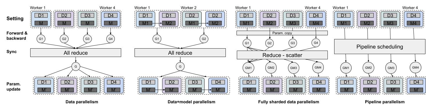
Data Parallelism

Data parallelism is the most common starting point.

• Every GPU keeps a full copy of the model.
• The batch is split into smaller mini-batches.
• Each GPU runs forward and backward on its own mini-batch.
• Gradients are synchronized across GPUs before the optimizer step.

If GPU 1 sees batch shard $B_{1}$ and GPU 2 sees batch shard $B_{2}$, both compute their own local gradients, and then an all-reduce averages or sums them. After synchronization, all model copies stay identical.

Why it is useful:

• simple mental model,
• easy to scale when the model fits on one device,
• standard choice for many training jobs.

Main limitation:

• it does not help if one full model already exceeds single-GPU memory.

Model Parallelism

Model parallelism splits the model itself across devices.

The simplest version is layer-wise model parallelism:

• early layers live on GPU 1,
• later layers live on GPU 2,
• activations are passed from one GPU to the next.

This helps when one device cannot hold the whole model, but it introduces communication between devices during both forward and backward passes. One stage may also wait for another stage, so utilization can drop.

Data + Model Parallelism

In practice, large systems often combine both ideas:

• split the global batch across workers,
• split the model across GPUs inside each worker group.

This hybrid setup is common because data parallelism solves throughput while model parallelism solves memory.

One important variant is fully sharded data parallelism (FSDP):

• parameters, gradients, and optimizer states are sharded across GPUs,
• each GPU stores only part of the model state most of the time,
• shards are gathered when needed for compute and then reduced/scattered again.

Compared with plain data parallelism, FSDP is much more memory efficient, but it adds more communication.

How FSDP Works Step By Step

Consider a simple 3-layer MLP

$$ x \rightarrow L_1 \rightarrow L_2 \rightarrow L_3 \rightarrow \mathcal{L}, $$

with weights $W_{1}, W_{2}, W_{3}$ split across two GPUs. The exact sharding pattern can vary, but the key FSDP idea is always the same:

• each GPU permanently stores only its shard,
• before a layer is computed, the full parameter for that layer is reconstructed by all-gather,
• after backward, the full gradient is reduce-scattered back into shards.

Suppose GPU 1 stores $W_{1}$, $W_{2}^{(1)}$, $W_{3}^{(1)}$ and GPU 2 stores $W_{2}^{(2)}$, $W_{3}^{(2)}$.

Forward pass

For layer 1, if $W_{1}$ is local to GPU 1, it computes

$$ a_1 = xW_1. $$

For a sharded layer such as $W_{2}$, the system first reconstructs the full weight:

$$ W_2 = \text{all-gather}(W_2^{(1)}, W_2^{(2)}). $$

Then the layer is computed exactly as usual:

$$ a_2 = a_1 W_2. $$

The same happens for $W_{3}$:

$$ W_3 = \text{all-gather}(W_3^{(1)}, W_3^{(2)}), \quad a_3 = a_2 W_3. $$

After each layer finishes, the temporary full parameter can be discarded and each GPU keeps only its shard again.

Backward pass

Backward starts from the loss and moves from the last layer to the first, just as in ordinary backpropagation.

For layer 3, each GPU temporarily has the full $W_{3}$, together with the needed activations and incoming gradient $\frac{\partial \mathcal{L}}{\partial a_{3}}$. It computes the standard local formulas:

$$ \frac{\partial \mathcal{L}}{\partial W_3} = a_2^\top \frac{\partial \mathcal{L}}{\partial a_3}, \quad \frac{\partial \mathcal{L}}{\partial a_2} = \frac{\partial \mathcal{L}}{\partial a_3} W_3^\top. $$

Then FSDP applies reduce-scatter:

• gradients are summed across workers,
• the summed gradient is partitioned back into shards,
• GPU 1 keeps only $\frac{\partial \mathcal{L}}{\partial W_{3}^{(1)}}$ and GPU 2 keeps only $\frac{\partial \mathcal{L}}{\partial W_{3}^{(2)}}$.

The same pattern repeats for layer 2:

$$ \frac{\partial \mathcal{L}}{\partial W_2} = a_1^\top \frac{\partial \mathcal{L}}{\partial a_2}, \quad \frac{\partial \mathcal{L}}{\partial a_1} = \frac{\partial \mathcal{L}}{\partial a_2} W_2^\top. $$

Again, the gradient is reduce-scattered so each GPU keeps only its shard.

For layer 1, if it is not sharded, the backward step is just the ordinary one-device computation.

Optimizer step

Each GPU updates only the parameter shard it owns. Across all GPUs together, these shards still represent the same global parameter vector as the non-sharded model.

Why FSDP Gives The Same Result As Non-Parallel Training

FSDP changes where tensors are stored, not the mathematical function being computed.

The key invariant is:

• forward uses the full parameter of each layer,
• backward computes the full gradient of that layer,
• sharding happens only for storage and communication.

For the forward pass, the equivalence is immediate. After all-gather, the layer uses the exact same weight matrix $W$ as a single-device run, so it computes the exact same activation:

$$ a = xW. $$

For the backward pass, suppose worker $i$ computes its contribution $G_{i}$ to the gradient of one layer from its local batch shard. The true full-batch gradient is the sum over workers:

$$ \frac{\partial \mathcal{L}}{\partial W} = \sum_i G_i. $$

Reduce-scatter is mathematically just

$$ \operatorname{reduce\text{-}scatter}(G_1, \dots, G_n) = \operatorname{shard}\left(\sum_i G_i\right). $$

So FSDP stores only part of the summed gradient on each GPU, but the value is exactly the same as the corresponding shard of the full gradient from non-parallel training.

That is why FSDP is mathematically equivalent to ordinary training:

• the same full weights are used during computation,
• the same layerwise formulas are used in backpropagation,
• the same full gradient is produced before being redistributed into shards.

The difference is purely systems-level: memory is reduced by sharding, while communication cost increases because parameters and gradients must be gathered and scattered during training.

Pipeline Parallelism

Plain model parallelism often wastes time because later GPUs must wait for earlier GPUs during forward, and earlier GPUs must wait for later GPUs during backward.

Pipeline parallelism fixes that waiting problem by splitting both:

• the model into stages,
• the batch into smaller micro-batches.

Then different stages work on different micro-batches at the same time.

Simple 2-GPU example

Suppose:

• GPU 1 stores layers $L_{1}, L_{2}$,
• GPU 2 stores layers $L_{3}, L_{4}$,
• one large batch is split into 4 micro-batches: $MB_{1}, MB_{2}, MB_{3}, MB_{4}$.

In naive model parallelism, GPU 2 would sit idle until GPU 1 finishes processing the whole batch. In pipeline parallelism, as soon as GPU 1 finishes the forward pass of $MB_{1}$, it sends those activations to GPU 2 and immediately starts working on $MB_{2}$.

So the forward pass looks like an assembly line:

Here $F$ means forward pass. The colors mark different micro-batches. GPU 2 starts later, but once the pipeline is full, both GPUs stay busy most of the time.

Backward pass in the pipeline

Backward works the same way in reverse. As soon as GPU 2 finishes the loss and backward computation for one micro-batch, it sends the activation gradient back to GPU 1, which can immediately start backward for that same micro-batch.

So the backward stream looks like:

Here $B$ means backward pass. Between GPUs, pipeline parallelism communicates:

• activations during forward,
• activation gradients during backward.

1F1B schedule

A common schedule is called 1F1B: one forward, one backward. After a short warmup period, each stage alternates between one forward step for one micro-batch and one backward step for another micro-batch. This greatly reduces idle time compared with running all forwards first and all backwards later.

Conceptually, after warmup the schedule looks like

$$ \cdots \rightarrow F \rightarrow B \rightarrow F \rightarrow B \rightarrow \cdots $$

on each stage, but for different micro-batches.

Why pipeline parallelism is still correct

Pipeline parallelism changes the order of execution, but not the mathematics.

If the full batch is split into micro-batches, the total loss is the sum of micro-batch losses:

$$ \mathcal{L} = \sum_i \mathcal{L}(MB_i). $$

Therefore the total gradient is also the sum of the micro-batch gradients:

$$ \frac{\partial \mathcal{L}}{\partial W} = \sum_i \frac{\partial \mathcal{L}(MB_i)}{\partial W}. $$

So pipeline parallelism is mathematically equivalent to standard training. It only reorders when each micro-batch is processed so that more hardware stays busy.

Pipeline bubbles

Pipeline parallelism does not remove idle time completely.

• At the beginning, later stages are waiting for the first micro-batch to arrive.
• At the end, earlier stages may finish before later ones.

These idle regions are called pipeline bubbles. A standard way to shrink the bubble is to use more micro-batches, which keeps the pipeline fuller for a larger fraction of the training step.

The tradeoff is that more micro-batches can increase scheduling overhead and activation memory pressure.

Mental model

Pipeline parallelism is like an assembly line:

• stages are GPUs,
• micro-batches are items moving through the factory,
• the goal is to keep every station working instead of waiting.

Tensor Parallelism

Tensor parallelism splits one large matrix operation itself across devices instead of only splitting by layers.

For a matrix multiply such as

$$ Y = XW, $$

we can shard $W$ by rows or columns so each GPU computes only part of the result.

• Column split: each GPU computes a subset of output features.
• Row split: each GPU computes a partial contribution that must later be reduced.

This is especially useful in transformer-style models with very large linear layers, embeddings, and attention projections.

When To Use Which

• Data parallelism: best when the model fits on one GPU and you mainly need more throughput.
• Model parallelism: best when the model is too large for one GPU.
• Pipeline parallelism: useful when the model is naturally split into stages and you want better utilization than naive model parallelism.
• Tensor parallelism: useful when individual matrix multiplications are too large and need to be partitioned inside a layer.
• FSDP: useful when memory is the bottleneck and you are willing to trade more communication for lower memory use.

For LLMs, real systems usually combine several of these at once. A common pattern is data parallelism across nodes together with tensor or pipeline parallelism inside a node.

Common Activations

• ReLU: fast, widely used, $\mathrm{ReLU}(x)=\max(0, x)$.
• GELU: smooth alternative to ReLU (both keep positive inputs and suppress many negative inputs, but GELU does it continuously and probabilistically rather than with a hard cutoff at 0), common in transformers/LLMs, $\mathrm{GELU}(x)=x\Phi(x)\approx 0.5x\left(1+\tanh\left(\sqrt{\frac{2}{\pi}}(x+0.044715x^3)\right)\right)$.
• Sigmoid: $\sigma(x)=\frac{1}{1+e^{-x}}$.
• Tanh: $\tanh(x)=\frac{e^x-e^{-x}}{e^x+e^{-x}}$.

Rule of thumb: start with ReLU (general deep learning) or GELU (transformer-style models).

Typical Failure Modes

• Too small model: underfitting.
• Too large model with little data: overfitting.
• Poor initialization or learning rate: unstable training.
  • Symptoms: loss explodes to NaN, or oscillates wildly, or stays flat from the start.
  • Weight initialization: the goal is to keep each layer’s output variance roughly equal to its input variance, so signals neither explode nor vanish as they propagate through many layers.

    • Where the $1/d$ comes from (forward pass): consider one layer $y = Wx$ (ignoring bias and activation). A single output element is a sum:

      $$ y_j = \sum_{i=1}^{d_{in}} W_{ji}\, x_i $$

      If the $W_{ji}$ and $x_{i}$ are independent and zero-mean, then:

      $$ \mathrm{Var}(y_j) = d_{in}\cdot\mathrm{Var}(W)\cdot\mathrm{Var}(x) $$

      To keep $\mathrm{Var}(y)=\mathrm{Var}(x)$ we need $\mathrm{Var}(W)=\frac{1}{d_{in}}.$

    • Where the $1/d$ comes from (backward pass): the gradient flowing back to each input element is:

      $$ \frac{\partial L}{\partial x_i}=\sum_{j=1}^{d_{out}} W_{ji}\,\frac{\partial L}{\partial y_j} $$

      This is a sum of $d_{out}$ terms (gradients flow through $W^T$). By the same variance argument:

      $$ \mathrm{Var}\!\left(\frac{\partial L}{\partial x_i}\right)=d_{out}\cdot\mathrm{Var}(W)\cdot\mathrm{Var}\!\left(\frac{\partial L}{\partial y}\right) $$

      To keep gradient variance stable across layers we need $\mathrm{Var}(W)=\frac{1}{d_{out}}.$

    • Forward pass vs. backward pass: the forward pass computes the prediction from input; the backward pass computes gradients from the loss back to each weight:

      $$ \text{Forward: } x \to h_1 \to h_2 \to \cdots \to \hat{y} \to \text{loss} $$

      $$ \text{Backward: } \frac{\partial L}{\partial \hat{y}} \to \frac{\partial L}{\partial h_2} \to \cdots \to \frac{\partial L}{\partial W} $$

      Weight variance needs to be controlled in both directions to keep signals and gradients stable.

    • Xavier/Glorot init (for Sigmoid/Tanh): compromises between forward ($1/d_{in}$) and backward ($1/d_{out}$) by averaging:

      $$ \mathrm{Var}(W)=\frac{2}{d_{in}+d_{out}}, \quad W_{ij}\sim\mathcal{N}\!\left(0,\;\frac{2}{d_{in}+d_{out}}\right) $$

      This assumes a near-linear activation around zero (which Sigmoid/Tanh approximate for small inputs).

    • He init (for ReLU, kaiming_normal_ in PyTorch): ReLU zeros out roughly half of the activations, so only about $d_{in}/2$ terms contribute non-zero values. To compensate, the variance is doubled:

      $$ \mathrm{Var}(W)=\frac{2}{d_{in}}, \quad W_{ij}\sim\mathcal{N}\!\left(0,\;\frac{2}{d_{in}}\right) $$

    • Why not all zeros? Every neuron computes the same output, so every gradient is identical, and the network can never break symmetry (it effectively has only one neuron per layer). Why not large random values? For Sigmoid/Tanh, large pre-activations push $e^{-x}$ toward $0$ or $\infty$, saturating outputs at their extremes (0/1 for Sigmoid, $\pm 1$ for Tanh) where gradients $\to 0$, so learning stalls (vanishing gradients). For ReLU and other unbounded activations, large weights cause activations to grow unchecked through layers, quickly reaching NaN (exploding activations).

  • Learning rate: start with a moderate value (e.g., $10^{-3}$ for Adam, $10^{-2}$ for SGD). If loss diverges, reduce by 10x. If loss barely moves, increase by 2–5x. A learning-rate finder (sweep from $10^{-5}$ to $1$ and plot loss) is a quick diagnostic.
  • Practical tip: combine a good initializer with Adam optimizer and a small learning rate as a safe default; tune from there.
• No normalization/regularization: weak generalization.
  • Symptoms: training loss is low but validation loss is much higher (large gap).
  • Normalization: apply Batch Normalization (BatchNorm) between layers for standard MLPs; it stabilizes activations and often speeds up convergence. For very small batch sizes or sequence models, Layer Normalization (LayerNorm) is preferred (and is the standard inside transformers).
  • Regularization options:
    • Dropout (e.g., rate 0.1–0.5): randomly zeros activations during training; simple and effective.

    - Weight decay / L2 (e.g., $\lambda=10^{-4}$): penalizes large weights; built into most optimizers (`weight_decay` in AdamW).

    - Early stopping: monitor validation loss and stop when it starts increasing.
- Rule of thumb: start with BatchNorm + Dropout (0.1–0.3) + weight decay ($10^{-4}$). Add or remove based on the train/validation gap.

Key Takeaways

Without activation, depth is useless. Stacking linear layers without nonlinearity collapses to a single linear mapping. The activation function is what gives depth its power: each layer can carve out a new decision boundary that the previous layer could not represent.

Backpropagation is just the chain rule applied in reverse. The core object is the vector-Jacobian product (VJP), not the Jacobian itself. You never compute or store the full Jacobian; you multiply each layer’s local Jacobian by the upstream gradient vector. This keeps memory and compute at $O(p)$ per layer instead of $O(p^2)$.

Forward-mode is cheap for one parameter, backward-mode is cheap for one loss. Forward-mode AD computes the gradient of all outputs with respect to one input in one pass. Backward-mode computes the gradient of one scalar loss with respect to all parameters in one pass. Since training has one loss and millions of parameters, backward-mode wins by a factor of $p$.

Track tensor shapes religiously. Most bugs in neural network code are shape mismatches. At every layer boundary, write down the shape: $(B, d_{\text{in}}) \to (B, d_{\text{out}})$. When a shape error occurs, printing the shape of every tensor at the failing line almost always reveals the problem immediately.

Parallelism strategies solve different bottlenecks. Data parallelism solves throughput (model fits on one GPU, need more speed). Model/pipeline parallelism solves model size (too large for one GPU). Tensor parallelism solves layer size (individual matrix multiplications too large). FSDP solves memory (shard optimizer state across devices). Real LLM training combines several of these simultaneously.

Initialization sets the trajectory. Xavier for sigmoid/tanh, He for ReLU. The goal is always the same: keep each layer’s output variance roughly equal to its input variance, so signals neither explode nor vanish across depth. Bad initialization (all zeros, too large) can make training impossible regardless of optimizer choice.

Tradeoff: model capacity vs generalization. More layers and wider hidden dimensions increase the function class the MLP can represent, but also increase the risk of overfitting. A model that is too small underfits (cannot capture the pattern); a model that is too large memorizes the training data (low training loss, high validation loss). Regularization (dropout, weight decay, early stopping) shifts the boundary, letting you use larger models without as much overfitting.

Tradeoff: communication vs memory in distributed training. Data parallelism replicates the full model on every device (high memory, low communication). FSDP shards the model across devices (low memory, high communication because weights must be gathered before each forward/backward pass). Pipeline parallelism sits in between: each device holds a portion of the model, but idle “bubble” time is the cost. The right choice depends on whether memory or bandwidth is your bottleneck.

Tradeoff: depth vs width. A deep, narrow network can represent hierarchical features but is harder to train (vanishing gradients, longer backpropagation chains). A shallow, wide network is easier to optimize but needs exponentially more parameters to represent the same hierarchical functions. In practice, moderate depth (2-4 layers for MLPs) with sufficient width is the sweet spot for most tasks.

Mini Checklist

Before training an MLP, decide:

1. Input feature design.
2. Number of layers and hidden size.
3. Activation function.
4. Loss and optimizer.
5. Evaluation metric.

Next Post

In Series 2, we will go deeper into training details: loss functions, full backpropagation derivations, and practical regularization tricks.

Ying Zhang

Ride with Uncertainties.

Additional author: WenboGuo

Tweet Share